이미지 인식(MLP, CNN)

1. 시작하며

기계학습, 딥러닝 카테고리에서는 관련 정보를 순서 대로 올리기보단 발췌하듯 글을 작성하고자 한다.

 

첫 번째 주제는 간단한 이미지 인식이다.

해당 내용은 "모두의 딥러닝(조태호)" 제 3판을 참고하여 작성하였다.

또 실습 환경은 Google Colab을 활용하였다.

 

2. 기초 인식(MLP 활용)

2.1. 사용 모듈

 

from tensorflow.keras.models import Sequential
from tensorflow.keras.layers import Dense
from tensorflow.keras.callbacks import ModelCheckpoint, EarlyStopping
from tensorflow.keras.datasets import mnist
from tensorflow.keras.utils import to_categorical
import tensorflow as tf

import matplotlib.pyplot as plt
import numpy as np
import os

2.2. MNIST 데이터 불러오기

# 데이터 불러오기
# 불러오는 형태는 format화 되어있다.
(X_train, y_train), (X_test, y_test) = mnist.load_data()

# 불러온 데이터 확인
print(f"학습셋 이미지 수: {X_train.shape[0]}개")
print(f'테스트셋 이미지 수: {X_test.shape[0]}개')

# 결과
"""
Downloading data from https://storage.googleapis.com/tensorflow/tf-keras-datasets/mnist.npz
11490434/11490434 [==============================] - 0s 0us/step
학습셋 이미지 수: 60000개
테스트셋 이미지 수: 10000개
"""

MNIST 자체에서 학습 데이터 수는 60000개, 테스트 데이터 수는 10000개로 저장해 놓았음을 알 수 있다.

 

2.3. 이미지 확인

# 이미지 확인
plt.imshow(X_train[0], cmap = 'Greys')
plt.show()

 

이미지를 불러 왔을 때 결과이다. 

2.4. 데이터 분리

# X_train.shape : (60000, 28, 28) -> reshape 후 (60000, 784)
# 255 나눗셈으로 0~1 사이 정규화를 진행해 주기 위해 타입을 실수로 변경한다.
# 데이터 폭이 클 때 적절한 값으로 분산의 정도를 바꾸는 과정을 데이터 정규화 라고 한다.
X_train = X_train.reshape(X_train.shape[0], X_train.shape[1]*X_train.shape[2]).astype('float64')/255
X_test = X_test.reshape(X_test.shape[0], X_test.shape[1]*X_test.shape[2]).astype('float64')/255

# 카테고리 변수로 변경한다. one-hot encoding 2 -> [0,0,1,0,0,0,0,0,0,0]
y_train = to_categorical(y_train, 10)
y_test = to_categorical(y_test, 10)

주석을 참고하면 충분히 이해 가능하다.

 

2.5. 모델 구조 설정

model = Sequential()
model.add(Dense(512, input_dim = 784, activation = 'relu'))
model.add(Dense(256, input_dim = 512, activation = 'relu'))
model.add(Dense(10, activation = 'softmax'))
model.summary()

2.6. 모델 실행 환경 설정

# 모델 실행 환경 설정
model.compile(loss = 'categorical_crossentropy', optimizer = 'adam', metrics = ['accuracy'])

# 모델 최적화를 위한 구간 설정
model_path = './MNIST_MLP.hdf5'

checkpointer = ModelCheckpoint(filepath = model_path, monitor = 'val_loss', verbose = 1, save_best_only = True)
early_stopping_callback = EarlyStopping(monitor = 'val_loss', patience = 10)

 

2.7. 모델 실행

tf.config.run_functions_eagerly(True)
history = model.fit(X_train, y_train, validation_split = 0.25, epochs = 50, batch_size = 200, verbose = 0, callbacks = [early_stopping_callback, checkpointer])

tf.config.run_functions_eagerly(True) 는 위의 코드 없이 실행했을 때 오류 같은 메세지로 떠서 추가하였다.

 

2.8. 결과 확인 및 시각화

# 검증셋과 학습 셋의 오차를 저장한다.
y_vloss = history.history['val_loss']
y_loss = history.history['loss']

# 그래프로 표현한다.
x_len = np.arange(len(y_loss)) # y_loss 길이 만큼 즉 epoch의 수만큼 x 축 길이를 설정한다.
plt.plot(x_len, y_vloss, marker = '.', c = 'red', label = 'Testset_loss')
plt.plot(x_len, y_loss, marker = '.', c= 'blue', label = 'Trainset_loss')

# 그리드를 주고 레이블을 표시한다.
plt.legend(loc = 'upper right') # 범례를 오른쪽 위에 표시한다.
plt.grid()
plt.xlabel('Epoch')
plt.ylabel('Loss')
plt.show()

print(f"\n Test Accuarcy: {model.evaluate(X_test, y_test)[1]:.4f}")

 

2.9. 통합

위의 과정을 class로 한번 통합해 보았다. 올바른 정리 법이라 할 순 없을 것이지만 class를 활용함에 의의를 두었다.

class MLP_classifier():

  def __init__(self,):
    (X_train, y_train), (X_test, y_test) = mnist.load_data()

    self.X_train = X_train
    self.y_train = y_train

    self.X_test = X_test
    self.y_test = y_test


  def data_processing(self, ):

    self.X_train = self.X_train.reshape(self.X_train.shape[0], self.X_train.shape[1]*self.X_train.shape[2]).astype('float64')/255
    self.X_test = self.X_test.reshape(self.X_test.shape[0], self.X_test.shape[1]*self.X_test.shape[2]).astype('float64')/255
    self.y_train = to_categorical(self.y_train, 10)
    self.y_test = to_categorical(self.y_test, 10)

  def model_define(self, ):
    model = Sequential()
    model.add(Dense(512, input_dim = 784, activation = 'relu'))
    model.add(Dense(256, input_dim = 512, activation = 'relu'))
    model.add(Dense(10, activation = 'softmax'))

    # 모델 실행 환경 설정
    model.compile(loss = 'categorical_crossentropy', optimizer = 'adam', metrics = ['accuracy'])

    return model

  def train(self):
    # 데이터 preprocessing 및 모델 정의
    self.data_processing()
    model = self.model_define()

    model_path = './MNIST_MLP2.hdf5'

    checkpointer = ModelCheckpoint(filepath = model_path, monitor = 'val_loss', verbose = 1, save_best_only = True)
    early_stopping_callback = EarlyStopping(monitor = 'val_loss', patience = 10)

    tf.config.run_functions_eagerly(True)
    history = model.fit(self.X_train, self.y_train, validation_split = 0.25, epochs = 50, batch_size = 200, verbose = 0, callbacks = [early_stopping_callback, checkpointer])

    self.model = model
    self.history = history

  def display_result(self):

    print(f"\n Test Accuarcy: {self.model.evaluate(self.X_test, self.y_test)[1]:.4f}")

    # 검증셋과 학습 셋의 오차를 저장한다.
    y_vloss = self.history.history['val_loss']
    y_loss = self.history.history['loss']

    # 그래프로 표현한다.
    x_len = np.arange(len(y_loss)) # y_loss 길이 만큼 즉 epoch의 수만큼 x 축 길이를 설정한다.
    plt.plot(x_len, y_vloss, marker = '.', c = 'red', label = 'Testset_loss')
    plt.plot(x_len, y_loss, marker = '.', c= 'blue', label = 'Trainset_loss')

    # 그리드를 주고 레이블을 표시한다.
    plt.legend(loc = 'upper right') # 범례를 오른쪽 위에 표시한다.
    plt.grid()
    plt.xlabel('Epoch')
    plt.ylabel('Loss')
    plt.show()
    
  
mlp_cls = MLP_classifier()
mlp_cls.train()
mlp_cls.display_result()

Random seed를 고정하지 않아 결과는 약간 다르나 비슷한 결과임을 확인할 수 있다.

 

3. CNN 활용

3.1. 사용 모듈

from tensorflow.keras.models import Sequential
from tensorflow.keras.layers import Dense, Dropout, Flatten, Conv2D, MaxPool2D
from tensorflow.keras.callbacks import ModelCheckpoint, EarlyStopping
from tensorflow.keras.datasets import mnist
from tensorflow.keras.utils import to_categorical
import tensorflow as tf
import matplotlib.pyplot as plt
import numpy as np

3.2. 데이터 불러오기

# 데이터 불러오기
(X_train, y_train), (X_test, y_test) = mnist.load_data()
X_train = X_train.reshape(X_train.shape[0], X_train.shape[1], X_train.shape[2], 1).astype('float64')/255
X_test = X_test.reshape(X_test.shape[0], X_test.shape[1], X_test.shape[2], 1).astype('float64')/255
y_train = to_categorical(y_train, 10)
y_test = to_categorical(y_test, 10)

3.3. 모델 구조 설정

#Convolution network 설정
model = Sequential()
model.add(Conv2D(32, kernel_size = (3,3), input_shape = (28,28,1), activation = 'relu'))
model.add(Conv2D(64, (3,3), activation = 'relu'))
model.add(MaxPool2D(pool_size = (2,2))) # (2,2) 풀링 창을 통해 max pooling 진행 최대값 저장
model.add(Dropout(0.25))
model.add(Flatten())
model.add(Dense(128, activation = 'relu'))
model.add(Dropout(0.25))
model.add(Dense(10, activation = 'softmax'))

3.4. 모델 확인

model.summary()
# param1 => 9*32+32(bias = channel 수)
# param2 => 32*64*9(32개의 이전 output과 64개의 channel연결, 각 채널 9개의 값 가짐)+64(bias = channel 수)
# maxpooling은 사이즈 줄이기, 파라미터 없음. (2,2) 사이즈 -> 넓이 1/2
# flatten -> 12*12*64

3.5. 모델 실행 전 설정

# 모델 실행 옵션 설정
model.compile(loss = 'categorical_crossentropy', optimizer = 'adam', metrics = ['accuracy'])

# 모델 최적화를 위한 설정
modelpath = "./MNIST_CNN.hdf5"
checkpointer = ModelCheckpoint(filepath = modelpath, monitor = 'val_loss', verbose =1, save_best_only = True)
early_stopping_callback = EarlyStopping(monitor = 'val_loss', patience = 10)

3.6. 모델 실행 및 시각화

# 모델 실행
#tf.data.experimental.enable_debug_mode()
history = model.fit(X_train, y_train, validation_split = 0.25, epochs = 30, batch_size = 200, verbose = 0, callbacks = [early_stopping_callback, checkpointer])

# 테스트 정확도 출력
print(f"\n Test Accuarcy: {model.evaluate(X_test, y_test)[1]:.4f}")

# 검증셋과 학습 셋의 오차를 저장한다.
y_vloss = history.history['val_loss']
y_loss = history.history['loss']
# 그래프로 표현한다.
x_len = np.arange(len(y_loss)) # y_loss 길이 만큼 즉 epoch의 수만큼 x 축 길이를 설정한다.
plt.plot(x_len, y_vloss, marker = '.', c = 'red', label = 'Testset_loss')
plt.plot(x_len, y_loss, marker = '.', c= 'blue', label = 'Trainset_loss')

# 그리드를 주고 레이블을 표시한다.
plt.legend(loc = 'upper right') # 범례를 오른쪽 위에 표시한다.
plt.grid()
plt.xlabel('Epoch')
plt.ylabel('Loss')
plt.show()

verbose =1 로 설정하였기에 나오는 시행 결과들은 표시하지 않겠다.

3.7. 모델이 틀린 것 확인

# model이 test데이터에 대해 내놓는 답을 뽑아낸다.
"""
뽑아내는 결과는 길이가 10인 1d array 이며 각 값은 라벨에 속할 확률을 의미한다. 마지막 layer의
activation이 softmax였음을 기억하자.
"""
test_label = model.predict(X_test)

# 오답을 말한 경우 index를 기억한다.
wrong_label_idx = []

for idx, label in enumerate(test_label):
  # 답에서의 갑들중 np.argmax를 이용해 최대값의 index를 뽑아낸다.
  # 예를들어 입력이 [1,2,3,2,1]이면 결과는 2이다.
  label = np.argmax(label)
  if int(y_test[idx][label]) == 1: # 정답을 맞추었다면 argmax 결과 얻은 index의 값에 1이 있어야 한다.
    continue
  else:
    wrong_label_idx.append(idx)

test 데이터에 대한 accuarcy가 0.9902 이므로 10000개의 데이터중 98개를 틀렸다. wrong_label_idx의 길이가 98이므로 오답인 결과를 찾는 올바른 코드였음을 알 수 있다.

 

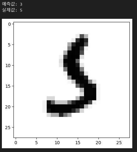
5개 정도 틀린 경우의 케이스를 확인해보자.

for i in range(5):

  idx = wrong_label_idx[i]

  # 이미지 확인
  print(f'예측값: {np.argmax(test_label[idx])}') # index 정보가 곧 숫자이므로. np.argmax를 통해 확률값이 제일 높은 수의 index 값을 찾는다.
  print(f"실제값: {np.argmax(y_test[idx])}")

  plt.imshow(X_test[idx], cmap = 'Greys')
  plt.show()

 

조금은 헷갈릴 만한 숫자들을 틀렸음을 확인할 수 있다.

 

4. 마무리하며

개념적인 부분 보다는 실습에 초점을 맞춘 것 같다. MLP와 CNN을 이용하긴 하였으나 단순한 적용이었기에 실제 적용을 위해 더 공부해야함을 느끼고 있다. 일단 16~21장까지 빠르게 정리하는 것이 목표이기에 정리 후 보다 deep하게 파볼 예정이다.

(추가: 책의 내용을 많이 참고한 것은 사실이나 주석에 본인의 생각을 적었고 책에 없는 내용을 추가하기도 하였으니 보다보면 도움이 될 내용이 있을 것이다. )